Blog-Series: SDE – Basics II: Spaces, Algebras & Measures

Definition of Stochastic Processes

Measure Spaces & Measures

Sigma Algebra

Measurable Space

Probability Space

Filtration

Literature

Definition of Stochastic Processes

Welcome to the second part of the Basic Concepts that is necessary for our Blog-Series. In this part, we will enhance the concept of spaces, introduce instruments to measure, and add probabilities to elements of spaces. Moreover, most importantly, we will start with the main question:

What is a Stochastic Process?

A stochastic process which is used in many fields and applications can be simply described as a collection of random variables, which is indexed by a set and be denoted by \left \{ X\left ( t \right ) \right \}_{t\in T}\left \{ X_{t} \right \}_{t\in T} , \left \{ X_{t} \right \}, or \left \{ X\left ( t \right ) \right \} In other words each random variable involved with the stochastic process is uniquely related with an element of its state space .

For demonstration purposes one can take a look at a realization of a stochastic process in the following (here an example of a random walk process, which will be introduced later in the blog-series).

Random Walk Realisation

As we have learned in the preceding blog post, a mathematical space can be seen as a set with a given structure.

State Space

A mathematical space can be defined by using integers, real lines, Euclidean or other (even complex) spaces. Values taken by the random variables are located in the same mathematical space, which is henceforth called the state space of a given random process.

The organization of the article is described in the following: Initially (as in the previous post), the whole concept will be presented. Secondly, a more mathematical rigor and detailed presentation of the underlying concepts and methods are taken into consideration. Nevertheless, proofs and complexities arising from too many fine details will be avoided and addressed in the literature.

At first, a definition of a Stochastic Process will be introduced:

Formal Definition of a Stochastic Process

A collection of random variablesdefined on a common Probability Space \left ( \Omega ,F, P \right ) is called a stochastic process, where

\Omega is a sample space
F or   \Sigma a \sigma – Algebra and
P is a probability measure

The random variables indexed by some set X indexiert , take values from the same mathematical space S , which must be measurable with respect to some \sigma – Algebra messbar . For a given probability space \left ( \Omega ,F, P \right ) and a Measurable Space \left ( S, \Sigma \right )
a stochastic process is a collection of S valued random variables, which can be written as:

\left \{ X\left ( t \right ): t \in T \right \}

while tdenotes a point in time T.

Before the given definition can be fully understood, it is necessary to present insights on the stated notations above. Since all of them are interrelated in some way, it is not possible to separate them entirely. Therefore, we use a “top-down” approach to get deeper into the topic. Even if some parts are explained later in the article, one can just thoroughly read and may accept some relevant terms to be introduced in the following steps of the article. We will start by introducing Measure Spaces next.

Measure Spaces & Measures

Zu Beginn ist es von Wichtigkeit zu erwähnen, dass Measure Spaces of Measurable Spaces zu unterscheiden sind. Daher, führen wir beide auch separat ein und sollten nicht verwechselt werden.

A Measurable Space contains information about the underlying set and comes into play if one is interested in the description of volumes. Subsets of the latter set can be measured using \sigma algebras (introduced in the following part of the article) and a methodology for measuring, namely a Measure. One example of a Measure Space is a Probability Space , also introduced later in the article.

Measurable Space

A Measure Space is a triple \left ( X, A, \mu \right ) , where

X is a non-empty set
 
A a \sigma – Algebra on X and
\mu
is a measure on \left ( X, A\right )

.

Since Measure Spaces are somehow related to volume, it makes sense to jump to the conclusion that volume can be measured to obtain information. Intuition tells us, that a volume can be seen as a size of some given object (e.g. the amount of air in a balloon). A measure on a set assigns a number to each suitable subset of a given set (which can be interpreted as size) and therefore can be seen as a generalization of the concepts of length, area and volume.

Measure

Let X be a set and \Sigma a \sigma – Algebra on X. A function \mu of \Sigma depicted to the extended real number line is called a measure if it satisfies the following properties :

  • Non-Negativity:  \forall E in \Sigma :\mu \left ( E \right )\geq 0

  • Non empty Set: \mu \left ( \varnothing \right )= 0

  • Countable Additivity: (also called \sigma– Additivity): For all countable collections \left \{ E_{j} \right \}_{j=1}^{\infty } of pairwise disjoint sets in \Sigma :
    \mu \left ( \bigcup_{k=1}^{\infty }E_{k} \right ) = \sum_{k=1}^{\infty }\mu \left ( E_{k} \right )

Some of the more commonly known measures are depicted in the following graphic:

Measures

In the next section, we will clarify the term of \sigma – Algebra , which plays an important role in this article.

Sigma Algebra

In the previous sections, the concept of a \sigma – Algebra is mentioned often, therefore it is time to introduce it properly. A \sigma – Algebra is a type of algebra of sets.

Algebra of Set

The algebra of sets defines the properties and laws of sets, the operations (e.g. calculation) of union, intersection, complementation and the relations of set equality and set inclusion. It needs to be closed under the union or intersection of finite subsets.

The terms union, intersection, complementation (basics of set theory) are explained in the following, using so called Venn-diagrams .

Union
Union
Intersection
Intersection
Absolute Complement
Complete Complement

A \sigma – Algebra (or \sigma field) is a type of Algebra of Set . On a set X , the \sigma – Algebra a collection C of Subsets of X , which X itself is included; it has to be closed under complement and under countable unions. In order to complement the former mentioned definition, the Empty Set has to be included as well and therefore a \sigma – Algebra needs to be closed under countable intersections too, indicating a stronger condition than the one of algebra of sets in general. Furthermore, a non-empty collection of sets is called a \sigma Ring. Because of this a \sigma – Algebra is a \sigma Ring that contains the universal set (Rings will not be discussed in this post any further).

Since the given explanation, sounds a little bit cryptic and one may be rattled by the thought of how many sets exist anyway to be counted, one important concept is introduced before going on, namely the notation of a Power Set.

Power Set

The set of all subsets of a given set X , including the empty set and X itself (measured by the "Weierstrass-p" is called the Power Set of X .

For a set X\left \{ a, b,c \right \} the following graphic shows the elements of the power set of X ordered with respect to inclusion (containment).

PowerSet
Elements of the Power Set of X

\sigma – Algebras are used in the definition of measures (which were introduced before). A collection of subsets for which a measure is defined, is therefore a \sigma – Algebra.

In general, sets can be formed from open or closed sets through upper mentioned operations, if the regarded space is a topological Space  T and are denoted as Borel sets . The collection of all Borel sets on T form a \sigma – Algebra (like noted in the paragraph before) which is known as Borel \sigma – Algebra since it is the smallest of all possible \sigma – Algebras on T containing all open (or closed) sets in T .

Let us now give a formal definition of a \sigma – Algebra to fully introduce this core concept :

Sigma – Algebra

Let  \Omega be a set, and a \sigma -Algebra F on  \Omega a collection of subsets of  \Omega with the following properties:

  • \varnothing \in F

  • \mathfrak{F}\in F\Rightarrow \overline{\mathfrak{F}}\in F, where \overline{\mathfrak{F}} = \Omega \setminus F be the complement of F in \Omega .

  • A_{1}, A_{2},… \in F \Rightarrow A:\bigcup_{j=1}^{\infty }A_{j}\in F

To finish the part about \sigma – Algebras it is worth mentioning that all elements of a \sigma – Algebra messbar are called measurable. This leads to our next section, namely Measurable Spaces.

Measurable Space

We have learned that we can measure sets and obtain information about it using \sigma – Algebras. Before going on, it is again worth mentioning that Measure Spaces are not to be confused with Measurable Spaces . Measure Spaces require a measure, which the Measurable Space does not .

Im Folgenden werden wir zunächst einen Measurable Space definieren.

Definition of a Measurable Space

The tuple \left ( X, A \right ) is called a measurable space, where

X is a nonempty set and

A a \sigma – Algebra on X .

To visualize this definition, it is worth to show some common measurable spaces, which are in some cases also called Borel Space.

We will now differentiate between two scenarios:

  • X is finite or countable infinite.

    In this case, the referring \sigma – Algebra corresponds to the power set on X . Therefore, A = P\left ( X \right ) and the measurable space can be written as \left ( X, P\left ( X \right ) \right ) .

  • X is a topological Space.

    In the second case (if compared with the definitions of a \sigma – Algebra in former part of the article), the \sigma – Algebra corresponds (in most cases) with the Borel \sigma – Algebra \mathfrak{B}. Therefore, A =\mathfrak{B} and the measurable space can be written as \left ( X, \mathfrak{B}\left ( X \right ) \right ) .

In scenario 2 we see, that topological spaces bear different attributes. Henceforth, the term Borel Space is either used synonymous to measurable spaces or spaces that are Borel isomorphic to a measurable subset in \mathbb{R} and lead to a Borel \sigma – Algebra .

Probability Space

Bis zu diesem Zeitpunkt haben wir sehr viel Wissen gesammelt. Nun werden wir das letzte unbesprochene Konzept erläutern, welches uns von einem vollumfänglichen Verständnis der Definition von stochastischen Prozessen am Anfang des Artikels abhält, nämlich Wahrscheinlichkeitsräume and Wahrscheinlichkeitsmaße.

Andrey Kolmogorov
Andrey Kolmogorov (1903-1987) is seen as the founding father of probability spaces.

Probability Measure

Is a Measure, which does not measure volumes orsizes(even if it needs to fulfil countable additivity properties), but instead must return results which are defined on the Unit Interval \left [ 0,1 \right ] .

Zero corresponds to the empty set and one to the whole space. In contrast to fuzzy measures (which are not part of this article), the assignment of one to equal the complete space under consideration is mandatory concerning probability measures.

In short, a probability measure is nothing else than the possibility of an event (or element) to occur, embodied by the entry probabilities ranging from zero (unlikely to happen) to one (certain to happen). Since these probabilities need a place to live (pun intended), probability spaces are a necessity, and are the next topic we will regard.

Probability Space

In der realen Welt (welche im Sinne dieses Artikels in weite Ferne entrückt scheint), treten Zustände (oder Szenarien, Ereignisse, Elemente) nicht deterministisch auf, sondern zufällig. Um diese zufallsgetriebene reale Welt zu modellieren, greifen Wissenschaftler und Forscher oft auf Modelle and Experimente zurück. Wenn man ein Experiment durchführt, (welches sich meist auf ein zugrundeliegendes Modell bezieht), sammeln wir Ergebnisse oder so genannte Ereignisse.

All events put together resemble the referring \sigma – Algebra F To know how probable certain of these events are, a Measurable Spaceis needed, namely a Probability Space.

A probability space consists of three parts:

  • A Sample Space \Omega , which contains all possible outcomes for a given model or experiment

  • F , the \sigma – Algebra, which resembles a set of events as described above

  • Probabilities, which indicate how certain (or not) an event is going to happen

In a Probability Space , a single outcome \omega from the sample space \Omega ) is selected and compared whether or which events in F verglichen, um zu bestimmen ob und wenn in welchen Elementen von F dieses contain contain the outcome. If the experiment is repeated often enough, one can see how often the outcome \omega occurs. Therefore, the probabilities can be functionally described.

Now we are able to mathematically define a probability space.

Formal Definition of a Probability Space

A Probability Space is a Measurable Space in dem das Maß des gesamten Raumes den Wert 1 annimmt (wie oben beschrieben). Man kann diese Definition wie folgt erweitern:

A probability space is a Triple \left ( \Omega ,F, P \right ) consisting of:

  • The Sample Space \Omega which is a nonempty set .


  • The \sigma – Algebra F\subseteq 2^{\Omega }also called a \sigma -field, which is a set of subsets of \Omega called events, in a manner that


    • F contains the Sample Space : \Omega \in F
    • F in regard of complements is closed : A \in F \Rightarrow \left ( \Omega \setminus A \right )\in F
    • F in regard of countable unions is closed : A_{j} \in F for j=1,2,…it is valid to note \left ( \bigcup_{j=1}^{\infty }A_{j} \right )\in F
    • Referring former points and the so called De Morgan´s Regel (not introduced in this article) F in regard of countable intersections is closed : A_{j} \in F for j=1,2,…it is valid to note \left ( \bigcap_{j=1}^{\infty }A_{j} \right )\in F


  • The Probability Measure P : F\rightarrow \left [ 0,1 \right ] needs to be a function on F such that:


    • P countable additive ( \sigma – additive) if \left \{ A_{j} \right \}_{j=1}^{\infty }\subseteq F is a countable collection of pairwise disjunct sets in a manner that P\left ( \bigcup_{j=1}^{\infty } A^{j}\right )=\sum_{j=1}^{\infty }P\left ( A_{j} \right )
    • P\left ( \Omega \right )=1

All concepts in the given definition were formally introduced earlier in this article and therefore will not be explained any further at this point. Additionally, one can review the definition of a stochastic process knowing all of the relevant terms involved.

To conclude this article, we are going to talk about filtrations in the final part.

Filtrations

When using \sigma – Algebras we can obtain information about the underlying sets and probabilities . As financial analysts, we are interested in the question when certain information is available in time.

A Filtration can therefore be seen as an increasing sequence of \sigma – Algebras in relation to some Probability Space and some index space . These have some total order relation , in most cases the index space is a T denoted representation of certain points in time .

Formal Definition of a Filtration

Let \left ( \Omega ,A, P \right ) be a probability space and let I be an index set with a total order \leq .

For all j \in I let F_{j} be a sub \sigma – Algebra of A .

Then  \mathbb{F}:=\left ( F_{j} \right )_{j\in I} is called a filtration, if F_{k}\subseteq F_{l}\subseteq A,\forall k\leq l gilt.

Filtrations are families of \sigma – Algebras that are ordered non decreasingly. If \mathbb{F} F is a filtration, then \left ( \Omega ,A,\mathbb{F}, P \right ) is called a filtered probability space.

Filtrations können genutzt werden um einen Überblick über die “set” (hier i.S.v. Anzahl, Masse an) an Informationen, welche einem stochastischen Prozess zu einem bestimmten Zeitpunkt zugrunde liegen, zu erhalten. Es wird angenommen, dass im Zeitablauf, der Informationsgehalt des Prozesses ansteigen wird.

With this in mind, the Basics for our Blog-Series is concluded. Our next article will follow the course of action presented in the introductory post of this series.

As always I am very thankful for feedback, indications and further questions.


Yours Respectfully,

Markus Vogl

Literature

Arens, T. et al., 2018. Mathematik. 4. Hrsg. s.l.:Springer.

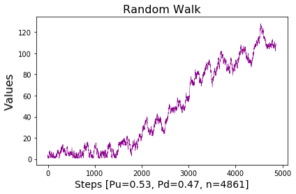
Gentle, J. E. (2002). Random Walks Ch.3. In J. E. Gentle, Elements of Computational Statistics (p. 41 von 420). Springer.

Gregory F. Lawler, V. L. (2010). Random Walk: A Modern Introduction. Cambridge Studies in Advanced Mathematics, Band 123.

Haugh, M. (2010). Introduction to Stochastic Calculus. Financial Engineering: Continuous-Time Models, 18.

Horst Rottmann, B. A. (2010). Statistik und Ökonometrie für Wirtschaftswissenschaftler – Eine anwendungsorientierte Einführung. Gabler.

James L. Cornette, B. S. (2004). Random walks in the history of life. PNAS, 187–191.

Klenke, A. (2008). Probability Theory. London: Springer.

Konstantopoulos, T. (2009). MARKOV CHAINS AND RANDOM WALKS. Introductory lecture notes. University of Liverpool.

Nelson, E. (August 2001). Dynamical Theories of Brownian Motion. Princeton University Press.

Oksendal, B. (2013). Stochastic Differential Equations – An Introduction with Applications. Springer.

Peter Mörters, Y. P. (März 2010). Brownian Motion. Cambridge Series in Statistical and Probabilistic Mathematics, Band 30.

Saloff-Coste, L. (2004). Random Walks on Finite Groups. Probability on Discrete Structures , pp 263-346.

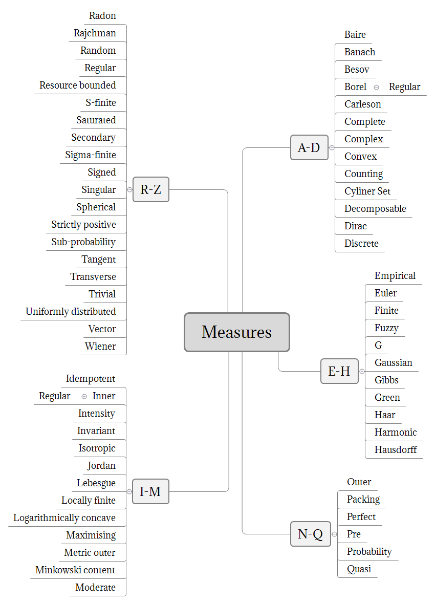
Sazonov, V. (2011, Februar 7). Encyclopedia of Mathematics. Retrieved from http://www.encyclopediaofmath.org/index.php?title=Measure&oldid=29871

Sousi, P. (October 2013). Advanced Probability. UK: University of Cambridge.

Szabados, T. (August 1994). An Elementary Introduction to the Wiener Process and Stochastic Integrals. Technical University of Budapest, 45.


Images and graphical content are taken from "wikimedia commons" database and are licensed using a CC-license if not states otherwise. If no reference is granted, the content belongs to the author.

Otherwise used Images and graphical content:

  • abstract painting art artistic von Anni Roenkae (Pexels Lizenz)